Chapter Hypothesis Testing with One Samples

§ 9.1 Null and Alternative Hypotheses

• `H_0`: the null hypothesis
  a statement about a population believed to be true
• `H_a`: the alternative hypothesis
  a claim about the population that differs from the null

Example:

Average weight of a U.S. male is at least 195 pounds*.
`H_0`: `mu=195`
`H_a`: `mu>195`

Example:
Most people don't forget their left-over box at a restaurant.
`H_0`: `p=0.5`
`H_a`: `p<0.5`

§ 9.2 Outcomes and Type 1 & 2 Errors

Possible outcomes

Action	`H_0` is Actually
	True	False
Do not Reject `H_0`	Correct Outcome	Type 2 error false negative
Reject `H_0`	Type 1 error false positive	Correct Outcome

---

Possible outcomes for: `H_0: mu<=0.003` oocysts/100L
safe level of Cryptosporidium in drinking water.
There are concerns over safe levels in a town's drinking water.
What are the concerns for possible errors

Test = Action	`H_0` is Actually
	True safe levels	False dangerous levels
Do not Reject `H_0` Test negative Water safe	Correct Outcome	Type 2 error false negative claim the water is safe, but it is not
Reject `H_0` Test Positive Water dangerous	Type 1 error false positive claim the water is not safe, but it is	Correct Outcome

§ 9.4 Unusual Events

Unusual Events

An event is considered unusual of the chance of something more extreme happening is low. Low is often a probability of less than 5%.

• If a person has a temperature of `101^circ F`, is this unusual?
  We believe that human body temperature has a mean of `98.6^circ F` and a standard deviation of `0.7^circ F`.
  I estimate the probability of a healthy person having a temperature greater than `101^circ F`, given that I expect `98.6^circ F` to be less than 1%. So a temperature of `101^circ F` is unusually high
• If a U.S. male has a weight of `100` pounds, is this unusual?
  We believe that U.S. male weight has a mean of `195` pounds and a standard deviation of `45` pounds.
  I estimate the probability of a healthy male having a weight less than `100` pounds, given that I expect `195` pounds to be about 2%. So, a male with a weight of `100` pounds is unusually low.

§ 9.5 The Hypothesis Test Procedure for a Mean

For a hypothesis test for a mean in StatKey we need the data, the null hypothesis, and the significance level.

1. Go to StatKey and select Randomization Hypothesis Tests: Test for  Single Mean.
2. Choose the appropriate data set, or select Edit Data to paste your own data in. Each number must be on its own line.
3. Enter the null hypothesis value.
4. Generate at least 5000 samples
5. Select the appropriate test: `square` Left tail, `square` Two tail, `square` Right tail
   1. Then enter the appropriate significance level: 0.025 or 0.05 or something else.
6. Make a decision:
   1. Is your sample mean in the red region (the critical region)? Yes? The Reject the Null
   2. Is your sample mean in the black region (the expected region)? Yes? Fail to reject the Null
7. Calculate the p-value.
   1. Replace the critical number with your sample mean. (the number below the significance level on the x-axis)
8. Re-affirm your decision based on the p-value:
   1. Is the p-value less than the significance level? Yes. Then definitely reject the null hypothesis
   2. Is the p-value greater than the significance level? Yes? Then fail to reject the null hypothesis

Example:

A realtor in Pendleton told me that the average home price is about $200K. Based on discussions with some newcomers to Pendleton, I thought it might be higher.

`H_0` : `mu=200,000` 
`H_a` : `mu>200,000`

I am going to choose a significance level of 5% since this is important, but not too important.

So I collect some data:

Home Prices, in thousands, Pendleton, OR, 2019
179.9	135.9	449	266	240
289.5	204.9	229	277.9	399
165	349.9	42	625	159.9
397	270	210	289	214.9
189	450	280	229	214.9
130	179.5	180	415	400
175	178.5	187	270	390
275	469.9	105	229.9	219
250	350	249.9	259.9	389.9
149.9	159	189	235	399

It is always a good idea to summarize the data before running a hypothesis test for a mean.

This is a reasonably large sample (n=50 > 30) and the histogram is a relatively symmetric bell shape with one large outlier, `(z=(625-264)/112~~3.223)`.

This sample seems to have a mean and median that are higher than $200,000, but is it significantly higher?

Enter the data into StatKey to get a sampling distribution to test the hypotheses: 
    Go to StatKey and select Randomization Hypothesis Tests: Test for  Single Mean.
    Edit Data to enter my data.
    Enter my null hypothesis value.
    Generate 1000s of samples.
    Select the Right Tail test.
    Enter my significance level.

Now draw this picture and label it:

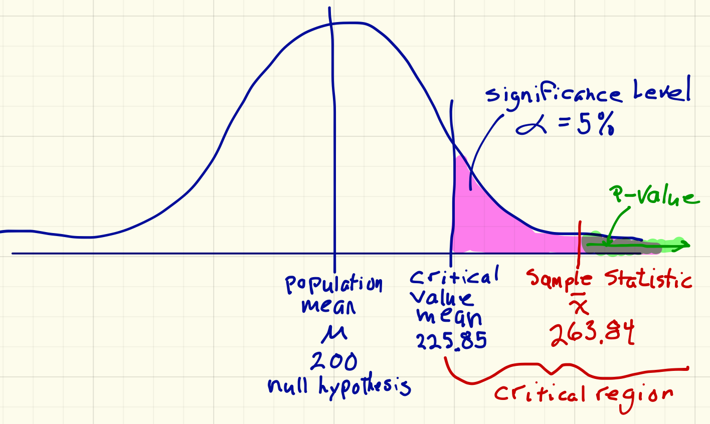
Now, reason through the decision and conclusion.

The mean of my sample, $263.84K is definitely in the red zone. The test is positive, i.e., I have evidence that the claim of the realtor is wrong.

To get the p-value, I then replace the critical number that StatKey gave me, 225.850, with my sample mean, 263.842.
According to StatKey, the p-value is 0.000. 

Interpretation of the p-value: `P(barx>263.84 \ | \ mu=200)`
The chance of finding another sample with a mean higher than $263.842K, assuming that the mean should be $200K, is almost 0.

Decision: Reject the null hypothesis.

Conclusion: We have sufficient evidence that the average home price in Pendleton is greater than $200 thousand.

§ 9.5 The Hypothesis Test Procedure for a Proportion

For a hypothesis test for a proportion in StatKey we need the sample size, the count of favorable occurrences, the null hypothesis, and the significance level.

1. Go to StatKey and select Randomization Hypothesis Tests: Test for Single Proportion.
2. Choose the appropriate data set, or select Edit Data to enter your own count and sample size.
3. Enter the null hypothesis value.
4. Generate at least 5000 samples
5. Select the appropriate test: `square` Left tail, `square` Two tail, `square` Right tail
   1. Then enter the appropriate significance level: 0.025 or 0.05 or something else.
6. Make a decision:
   1. Is your sample proportion in the red region (the critical region)? Yes? The Reject the Null
   2. Is your sample proportion in the black region (the expected region)? Yes? Fail to reject the Null
7. Calculate the p-value.
   1. Replace the critical number with your sample proportion. (the number below the significance level on the x-axis)
8. Re-affirm your decision based on the p-value:
   1. Is the p-value less than the significance level? Yes. Then definitely reject the null hypothesis
   2. Is the p-value greater than the significance level? Yes? Then fail to reject the null hypothesis

Example:

In a recent survey by The Economist magazine, President Trump's approval rating is estimated to be about 42%.
A random sample of 50 North-East Oregon residents had 24 who approve of the Presidents performance.

`H_0` : `p=0.42` 
`H_a` : `p!=0.42` 

Although I could have picked an alternative hypothesis of >, I chose not equal instead.

I am going to choose a significance level of 5% since this is important, but not too important.

Enter the data into StatKey to get a sampling distribution to test the hypotheses: 
    Go to StatKey and select Randomization Hypothesis Tests: Test for  Single Proportion
    Edit Data to enter my count, `x=24` , and sample size, `n=50` .
    Enter my null hypothesis value.
    Generate 1000s of samples.
    Select the Two Tail test.
    Enter my significance level.

My sample proportion, 0.48, is not in the red zone. The test is negative, i.e., I do NOT have evidence that Economist's estimate is different in Eastern Oregon.

To get the p-value, I then replace the right critical number that StatKey gave me, 0.56, with my sample proportion, 0.48.

According to StatKey, the p-value is 0.474. In a two tail test, the p-value is the sum of both tails.

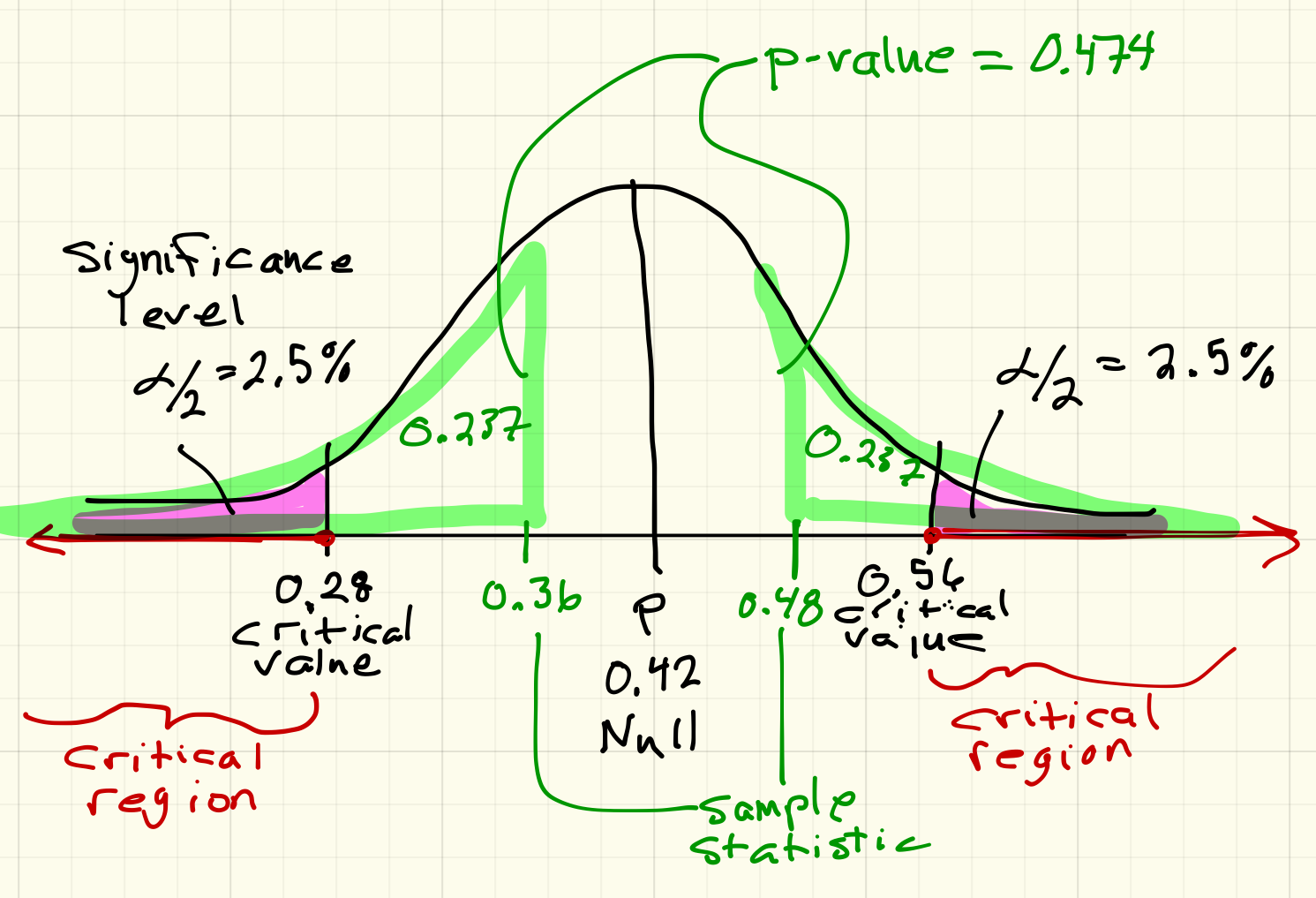
Interpretation of the p-value: The chance of finding another sample with a proportion higher than 0.48 or lower than 0.36, assuming that the actual proportion should be 0.42, is about 47.4%.

Decision: Fail to reject the null hypothesis.

Conclusion: We do NOT have sufficient evidence that the President's approval rating in North-Eastern Oregon is different than 42%.